Guided Intro to Using BadgerCompute

Welcome! This short, hands-on intro will get you running on BadgerCompute, UW–Madison’s JupyterHub service. You’ll:

Launch JupyterLab using the Basic Data Science container
Download a ready-made notebook and a small dataset
Run a toy analysis in Python using pandas and matplotlib
Save your work, shut down, and log out

Prerequisites

No local installs are required—everything runs in the cloud! This introduction assumes that

You have an active UW-Madison NetID
You have passed the BadgerCompute Certifcation Course and have waited 24 hours
You are using a modern web browser (Chrome/Firefox/Safari)

Log in and choose the notebook environment

Launch the BadgerCompute notebook service.
Log in with your UW credentials and accept the Terms if prompted.
On the "Server Option" page, choose the environment Basic Data Science.
Click the Start button to launch the notebook using that environment.

This may take a few minutes

Wait patiently while your server starts. If it takes more than 10 minutes, try refreshing the page or logging out and back in. Wait times may be longer during peak usage periods.

Familiarize yourself with JupyterLab's Interface

When notebook environment loads, you'll see the following components:

File Browser (left sidebar): navigate folders, upload/download files.
Launcher (main area): create new Notebooks/Terminals/Text files.
Notebook Apps: Open a notebook
Console Apps: Open an interactive console
Other Apps: Open a terminal or other interface

Notebook vs Console vs Terminal

A Notebook is a living document for your code, where you can write text alongside your actual code.
A Console is an interactive mode for entering commands in a particular programming language and provides a variety of enhancements, such as auto-complete suggestions and help text.
A Terminal is also an interactive mode for running commands but without the enhancements of the Console, which means it can run faster than the Console.

For reproducible work, most people use the Notebook because it allows you to save everything - the commands, the output, the instructions - as a single standalone file. The Console is good for testing and developing specific code, and the Terminal is good for running quick commands, but neither can easily save the work.

Create a workspace folder

Let’s keep this tidy:

In the File Browser, double-click on /work
Right-click and choose New Folder.
Name it: badgercompute_intro
Double-click to enter that folder.

Persistent storage

Your /work directory is the only top-level directory which offers persistent storage. Only the contents of the /work directory are kept between notebook sessions!

Be sure to read the BadgerCompute data policies.

Download a notebook and dataset

Next, you'll be guided on how to download:

An example notebook from a public repository
The "Palmer Penguins" dataset

You can do this using either a Terminal or a Notebook.

Option A: Use a Terminal

From the Launcher, under the Other section, click the Terminal app.
Make sure you are in right folder by running this command:
```
cd ~/work/badgercompute_intro
```
Download the example notebook by running this command:
```
wget -O getting_started.ipynb https://raw.githubusercontent.com/Reproducible-Science-Curriculum/introduction-RR-Jupyter/e5aece1011a43edfd739cbd83a2f4346091a86e2/notebooks/getting_started_with_jupyter_notebooks.ipynb
```
After the command finishes running, you should see the new getting_started.ipynb file in your file browser pane on the lefthand side (you may need to refresh the pane).

Similarly, download the "Palmer Penguins" dataset by running

wget -O penguins.csv https://raw.githubusercontent.com/allisonhorst/palmerpenguins/master/inst/extdata/penguins.csv

A new penguins.csv file should appear in your directory.

You can confirm the files exist by listing the contents of the current directory with this command:
```
ls -lh
```

Option B: Use a Notebook

From the Launcher, under the Notebook section, click the Python app.
Download the example notebook by pasting this command into the notebook cell, then running it using the Shift+Enter keyboard shortcut:
```
!wget -O getting_started.ipynb https://raw.githubusercontent.com/Reproducible-Science-Curriculum/introduction-RR-Jupyter/e5aece1011a43edfd739cbd83a2f4346091a86e2/notebooks/getting_started_with_jupyter_notebooks.ipynb
```
After the command finishes running, you should see the new getting_started.ipynb file in your file browser pane on the lefthand side (you may need to refresh the pane).

The ! at the start of the command is required to run a non-Python command inside of the Python notebook.

Similarly, download the "Palmer Penguins" dataset by running

!wget -O penguins.csv https://raw.githubusercontent.com/allisonhorst/palmerpenguins/master/inst/extdata/penguins.csv

A new penguins.csv file should appear in your directory.

You can confirm the files exist by listing the contents of the current directory with this command:
```
!ls -lh
```

Open the downloaded notebook

In the File Browser, double-click the file getting_started.ipynb to open it.

We highly encourage your to read through the notebook contents. The notebook was created by the Reproducible Science Curriculum team and is a great resource to learn more about Jupyter notebooks and basic Python.

Keyboard shortcuts for the notebook

Here are some frequently used shortcuts for interacting with Jupyter notebooks:

Shift Enter: run a cell
Esc then M: change cell type to Markdown
Esc then Y: change cell type to Code
A: insert cell above current cell
B: insert cell below current cell

Create your own notebook

Next, you'll be guided through making your own notebook for a small analysis.

Open a new Launcher tab by clicking the “+” icon in the tab bar.
Under Notebook, click on the "Python" app to open a new notebook.
Save the notebook - you'll be prompted to provide a name for the new file. Save it as toy_penguins_analysis.ipynb inside badgercompute_intro/.

Saving
You can save your notebook using the normal keyboard shortcut, or by going to "File" and cliking on "Save Notebook" in the menu bar.

Using Markdown in Your Notebook

You can add text cells using Markdown to explain your analysis.

To see this in action, copy the following text and paste it into the notebook cell.

# Meet the Penguins

For this toy tutorial, we will use the [Palmer Penguin dataset](https://allisonhorst.github.io/palmerpenguins/). 
The dataset was collected by [Kristen Gorman](https://www.uaf.edu/cfos/people/faculty/detail/kristen-gorman.php) and the [Palmer Station Antarctica Long Term Ecological Research Network](https://pallter.marine.rutgers.edu/).
![Artwork of a Chinstrap, Gentoo, and Adelie Penguin - Artwork by @allison_horst](https://allisonhorst.github.io/palmerpenguins/reference/figures/lter_penguins.png)

Artwork by @allison_horst

By default, the first cell in a new notebook is set to "Code" type, but you want this one to be the "Markdown" type. To convert a cell to Markdown, click the dropdown box at the top of the notebook that says Code and select Markdown. To edit the cell after changing it's type, double-click it.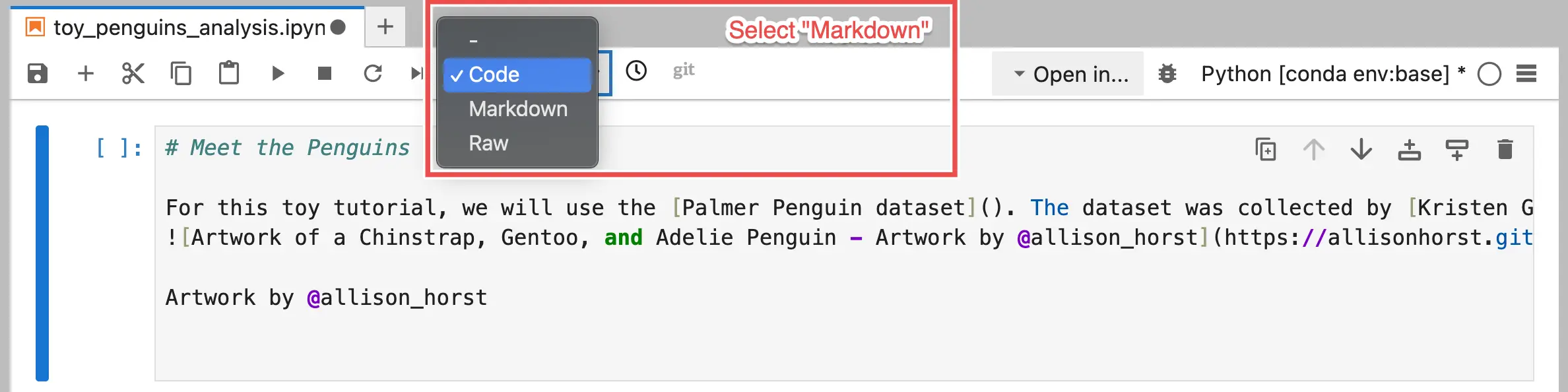

To render the Markdown into its pretty form, run the Markdown cell. This will also create a new Code cell below the rendered content.

Import libraries and load data

In the new code cell created by the previous step, copy and paste the following code:

import pandas as pd
import matplotlib.pyplot as plt
import seaborn as sns

# Load the CSV we downloaded
penguins = pd.read_csv("penguins.csv")
penguins.head()

Then run the cell to make the notebook execute the commands in that cell. You'll see the first few rows of the table loaded from the CSV file.

Inspect and clean

In one cell or in multiple cells, run the following code snippets to inspect and clean up the dataset you loaded:

# Quick shape and columns
penguins.shape, penguins.columns.tolist()

# Basic info and missing values
penguins.info()
penguins.isna().sum()

# Drop rows missing core numeric measurements to simplify this toy example
clean_penguins = penguins.dropna(subset=["bill_length_mm", "bill_depth_mm", "flipper_length_mm", "body_mass_g"])
clean_penguins.shape

The last command should return (342, 8).

Simple stats and grouping

The following code snippets calculates statistics for certain groups within the dataset. Again, run these commands in one or multiple cells in your notebook.

# Average bill length per species
clean_penguins.groupby("species")["bill_length_mm"].mean().round(2)

# Average body mass by species & sex
clean_penguins.groupby(["species", "sex"])["body_mass_g"].mean().round(1).unstack()

A quick plot

One of the powerful features of notebooks is the ability to display images in the same document as the code used to generate them.

Here, you'll use the pandas integration with matplotlib to generate several plots illustrating trends in the dataset. Run the following code snippets in your notebook to do so.

# Scatter: bill length vs. bill depth
ax = clean_penguins.plot.scatter(x="bill_length_mm", y="bill_depth_mm", title="Penguins: Bill Measurements")
plt.show()

# Histogram of flipper lengths
ax = clean_penguins["flipper_length_mm"].plot.hist(bins=20, title="Penguins: Flipper Length Distribution")
plt.xlabel("flipper_length_mm")
plt.show()

Compare between species

Next, you'll make a more elaborate plot.

# --------------------------------------------
# Bill length vs. depth with regression lines
# --------------------------------------------
plt.figure(figsize=(8,6))

sns.lmplot(
    data=penguins,
    x="bill_length_mm",
    y="bill_depth_mm",
    hue="species",
    palette=["darkorange", "purple", "#008B8B"],  # fixed
    height=6, aspect=1.2
)
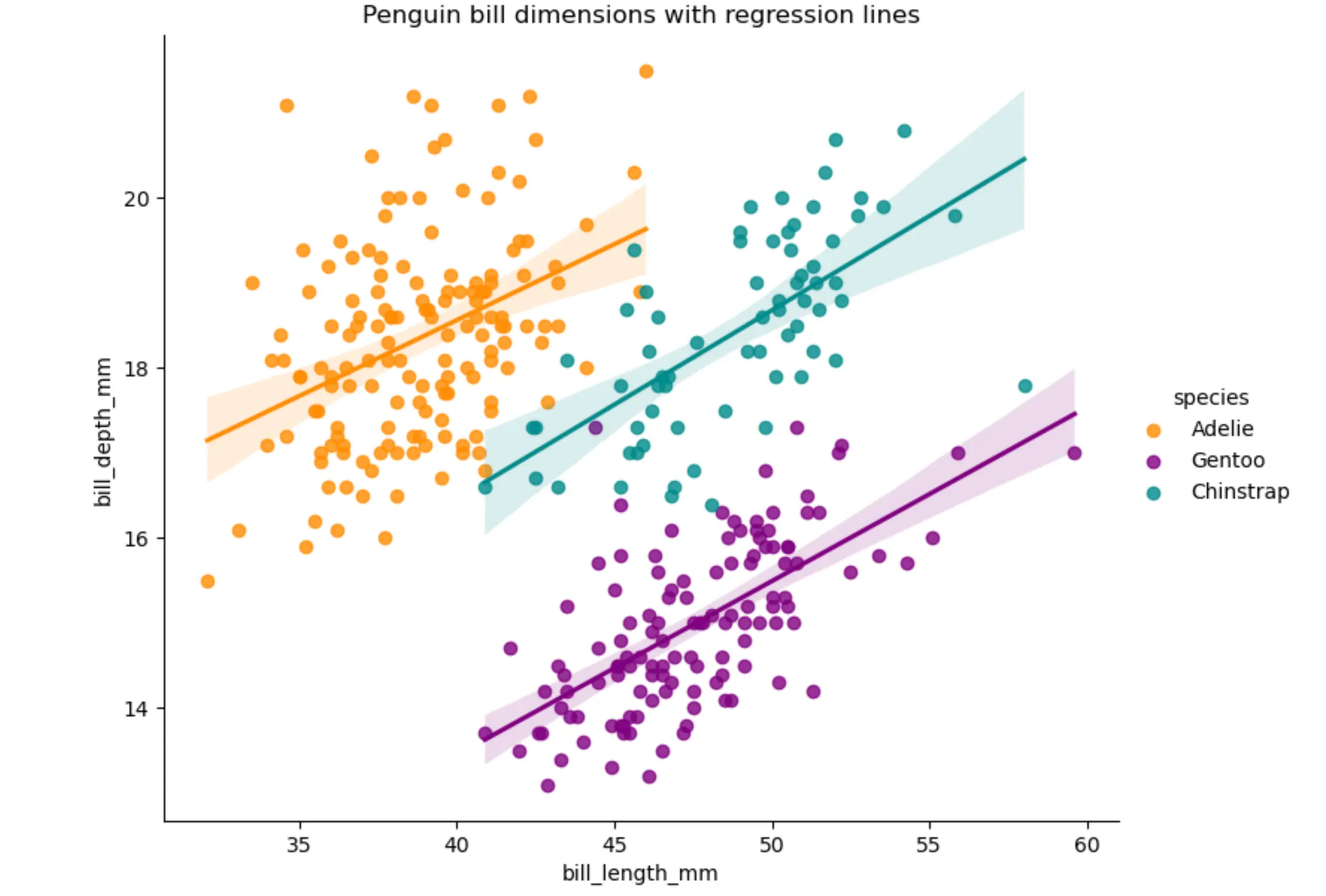
plt.title("Penguin bill dimensions with regression lines")
plt.show()

Your output plot should look something like this:

What if you wanted to change the color of the plot? All you have to do is change the contents of the code cell that generated plot, then re-run it. The plot will update with the changes.

If plots don’t render, make sure that all the cells ran without error and that you are using a Python notebook.

Annotate your notebook

Jupyter notebooks are great for mixing code, results, and narrative text. This makes them ideal for sharing and reproducible research. You can add Markdown cells to explain your steps.

If you aren't familiar with how to use Markdown syntax, we recommend reading the Jupyter Markdown Guide.

In addition to formatting text, you can also add images, LaTeX math, and more!

Save, restart, and export

When you are done editing the notebook, make sure to save it! We also recommend downloading a copy of the notebook to your own computer as a backup.

Save: File → Save Notebook
Restart Kernel: Kernel → Restart Kernel (useful if things get “stuck”)
Download: File (or right-click the file in the pane) → Download
Export: File → Save and Export Notebook As… (e.g., HTML)

File persistence and best practices

The contents of the /work directory are saved across BadgerCompute sessions, subject to the Data Retention Policy.

If you want to make sure you don't lose your data, we encourage you to download the files at the end of the session.

Shut down and log out

To end your BadgerCompute session, follow these steps:

Close notebooks or shut down their kernels from the Running Terminals and Kernels panel (left sidebar → “Running” tab).
Log out by going to File → Log Out.
Close your browser tab.

It's okay if you don't follow this procedure every time - the BadgerCompute session will automatically shut down after 10 minutes without any browsers open.

Forward - Where to go next

Explore more notebooks in your repo or public tutorials.
Try pandas joins/merges, groupby + aggregation, or matplotlib/plotly visualizations.
Practice uploading your own CSV via the File Browser and running similar analyses.

If you have questions or just want to chat about the possibilities, join the BadgerCompute Community Forum!

BadgerCompute